As we know traditional embedding models generate a single, fixed vector for each piece of data. This might creates a fundamental dilemma :
- large vectors (1536 dims) offer high accuracy, but they demand significant memory, compute power and of course money. sometimes they are an overkill for simple tasks and prohibitive for edge devices
- small vectors (64d) are efficient but sacrifice nuance and details needed for complex applications
This forces you with one of two choices : train and maintain multiple models for different needs, or accept a costly compromise in performance or efficiency
Classical trade-off :
| Vector Size | Pros | Cons |
|---|---|---|
| Small (300) | Fast & efficient, good for mobile devices. | Less detailed, might miss nuances, less accuracy |
| Large (1536) | Very detailed and high accuracy | Slower & requires powerful computers. |
What if i told you that you can have the best of both worlds without needing two separate models?
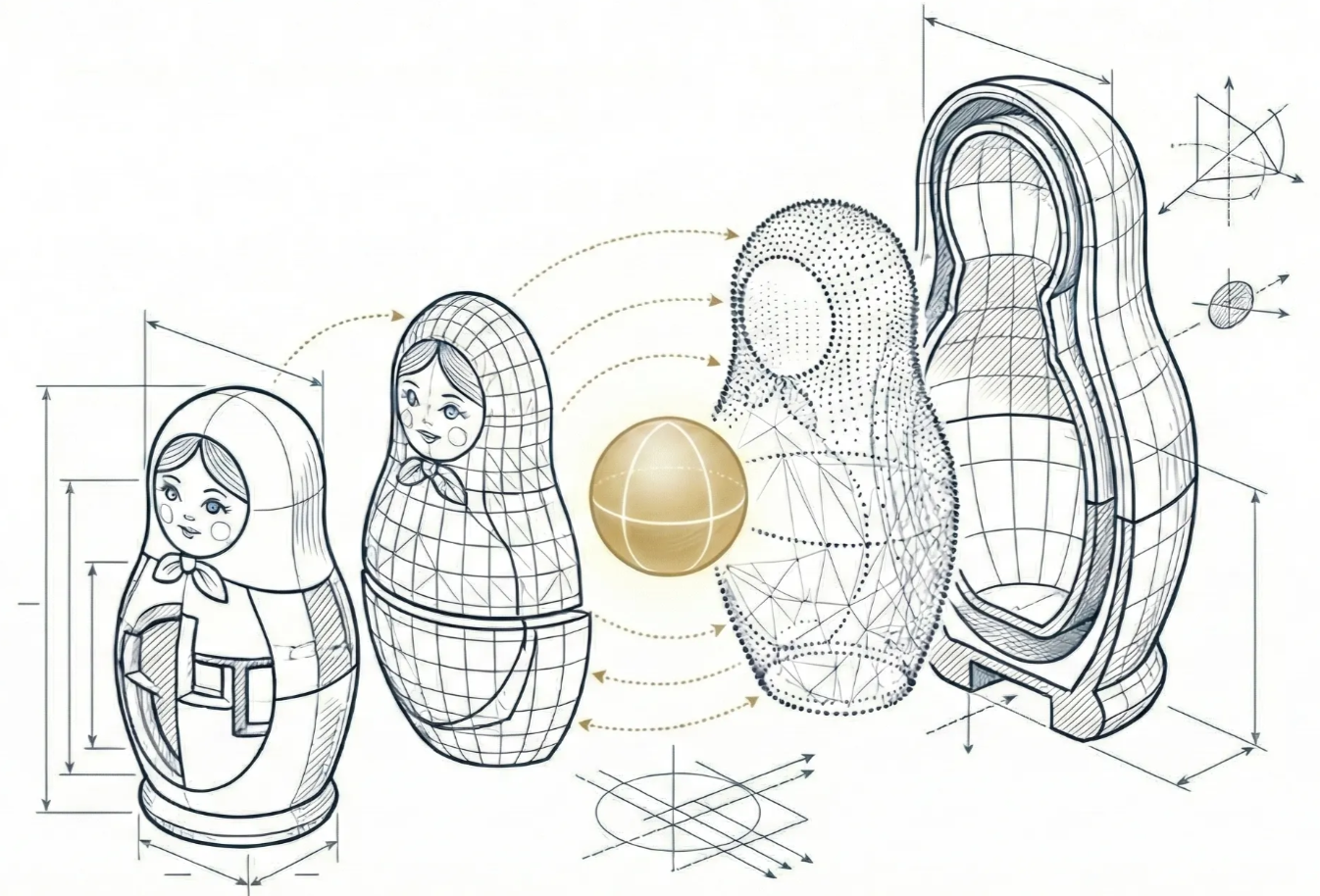
The matryoshka concept : one model, many resolutions
The matryoshka embeddings ‘Feb 2024 paper’ inspired from Russian nested dolls provide several nested vectors within a single output in which each layer adds a new level of complexity
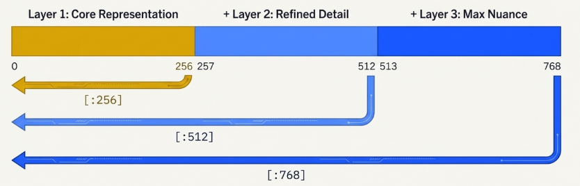
Layer 1 is simply first group of numbers from that list and each subsequent layer is progressively longer slice from the start of the same single vector, going from layer 1 to layer 2 we add more details or dimensions
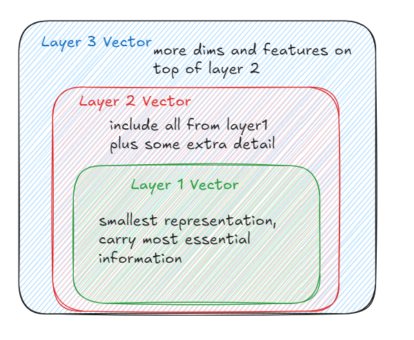
It is just logical partitioning: Physically a matryoshka embedding is just one large vector , so that the nesting is just a logical concept achieved by slicing the vector at a pre-defined points. the model is trained to ensure that even the first slice is independently meaningful and useful
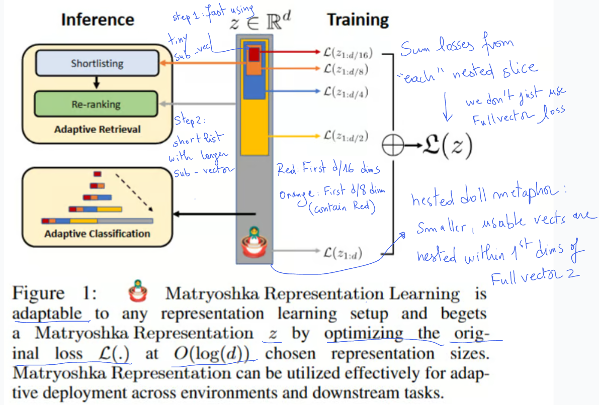
matryoshka representation learning MRL
It is as defined in the official paper a training strategy that forces subsections of an embedding to be independently useful and this is how it works
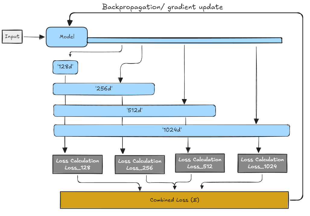
- during training, we define multiple dims (for eg: 128, 256, 512, 1024)
- the output is simply a full vector which then the system truncates it to each defined size and calculates a separate loss for each slice
- these losses then are summed. the model is penalized if any slice performs poorly on the task
If you try to do this [:, :256] slice on an older model (like the original BERT or text-embedding-ada-002), the resulting vector will perform very poorly because those models distribute information equally across the entire length of the embedding.
What MRL is NOT:
- It is not an inference optimization trick like pruning or quantization
- it does not make the model forward pass faster or lighter , it will compute the entire embedding vector
what MRL is :
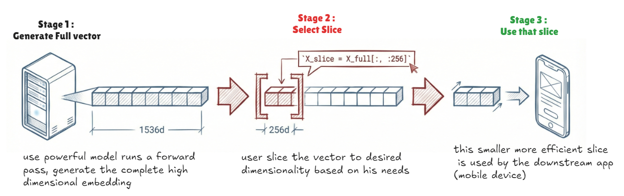
- It is about one powerful model which produce one large flexible embedding
- the magic happens after inference when you choose how much of the generated vector to use downstream
Key performance metrics (based on the official paper)
Classification : achieves same ImageNet accuracy as standard baselines but with up to 14X smaller embedding sizes
Retrieval : in adaptive retrieval settings MRL allows for up to 14X real world speedups by using small dims for a first pass (shortlisting) and larger dims for reranking with no loss in acc.
Accuracy : lower dimensional slices of MRL model often match or outperform independently trained of that specific size (MRL slice of 64 dims is as good as a model trained specifically to output 64 dims)
Adaptive retrieval
If you are trying to find a book in a 10 million book library you can choose between
Standard retrieval which is too slow cuz you have to pick up every single book read the summary (use the 2048 dims) and decide if it matches what you need
Adaptive retrieval (fast and smart ) it is a two steps funnel :
step 1 : shortlisting (pass 1 - the 128x speedup) : the analogy here when you are searching for that specific book you take a glance at the titles (which is in our case the 16d). you may ask why the title and MRL would answer that it is forcing the “title” to contain the most important info, which is obviously can let you reject more than 90% of the rest of the books. Then you grab for example 200 books that seems relevant.
The result : this is theoretically 128X faster because we processed very little data for the massive pile of the books
Step2 : the reranking (pass 2 )
we take those selected 200 books, and we read the full summary (the full 2048 dims) for only these books to find our perfect match
The result : when doing the heavy reading only on those 200 books it takes almost no time
OpenAI ‘text-embedding-3’ models
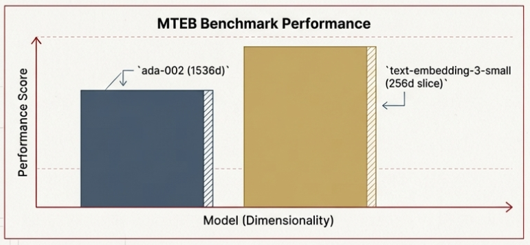
in early 2024 openAI tried MRL for its new “text-embedding-3-small ” and “text-embedding-3-large” models , which shows that a 256d slice can outperform a full 1536d vector
Matryoshka with Qdrant
Step1 : multi-step matryoshka retrieval
we just start the search with smallest fastest embedding slice for example 64d then progressively refine results by reranking with larger slices
from qdrant_client import QdrantClient, models
client = QdrantClient("http://localhost:6333")
# The first branch of our search pipeline retrieves 25 documents
# using the Matryoshka embeddings with multistep retrieval.
matryoshka_prefetch = models.Prefetch(
prefetch=[
# first retrieve 100 candidates using fastest(lowest) 64d slice
models.Prefetch(
prefetch=[
models.Prefetch(
query=[...],
using="matryoshka-64dim",
limit=100,
),
],
# secondly rerank those 100 using more accurate 128d slice.
query=[...],
using="matryoshka-128dim",
limit=25, # return final top 25
)
client.query_points("my-collection", prefetch=[matryoshka_prefetch], ...)stage 1 : is fast and broad, fast initial search retrieves 100 potential candidates using most efficient 64-dim slice
stage 2: accurate and focused , the sys then reranks using more detailed 256 dim slice returning top 25
- the entire operation happens server-side in Qdrant. It’s efficient cuz the expensive high dimensional comparison is only performed on a small subset of the data
Step 2 : Fusing with dense and sparse vectors
# The second branch of our search pipeline also retrieves 25 documents,
# but uses the dense and sparse vectors, with their results combined
# using the Reciprocal Rank Fusion.
sparse_dense_rrf_prefetch = models.Prefetch(
    prefetch=[
        models.Prefetch(
            prefetch=[
                # The first prefetch operation retrieves 100 documents
                # using dense vectors using integer data type. Retrieval
                # is faster, but quality is lower.
                models.Prefetch(
                    query=[...],
                    using="dense-uint8",
                    limit=100,
                )
            ],
            # Integer-based embeddings are then re-ranked using the
            # float-based embeddings. Here we just want to retrieve
            # 25 documents.
            query=[-1.234, 0.762, ..., 1.532],
            using="dense",
            limit=25,
        ),
        # Here we just add another 25 documents using the sparse
        # vectors only.
        models.Prefetch(
            query=models.SparseVector(
                indices=[...], values=[...],
            ),
            using="sparse",
            limit=25,
        ),
    ],
    # RRF is activated below, so there is no need to specify the
    # query vector here, as fusion is done on the scores of the
    # retrieved documents.
    query=models.FusionQuery(
        fusion=models.Fusion.RRF,
    ),
)
Dense and sparse vector search would get us each 25 docs and then with RRF (reciprocal rank fusion) we finally get a single relevance ranked list
Tip : for multi-vector models used only for reranking (like colbert ), disable HNSW graph creation (just set m=0 ) , this prevents indexing which is unnecessary and resource consumption
The big idea : matryoshka representation learning delivers a single, flexible vector that scales to your needs. one model can now serve both high powered servers and resource constrained devices
workflow : heavy lifting happens on powerful hardware , however at inference time we simply slice off the dimension you need.
where the metaphor of dolls bends (but doesn’t break )
- it is slicing not nesting : means that in code we are slicing a single large vector
(’myvec[:256])’),not physically opening separate dolls - the model learns all layers simultaneously during training unlike a doll build layer by layer
- fixed boundaries : slices are fixed at training time, and you can’t ask for a custom 400d slice without retaining
- the model may learn features that overlap across slices unlike the clean separation of physical doll
MRL offers a clever unified way to nest different levels of details inside a single embeddings space, which fundamentally changing how we approach efficiency and flexibility in AI. You get a single , flexible let’s call it elastic vector that can serve high powered servers and resource-limited edge devices. It is to be honest a clever way to nest different levels of detail inside one unified embedding space.
References
- Code Repo for MRL
- Matryoshka Representation Learning
- Qdrant Hybrid search Blog
- Qdrant Cloud Sign Up
- Subscribe to the Qdrant Newsletter

(END)