Qdrant 1.19: Turbo4 Datatype & Memory Tiers

One config line, nine times less disk, and a single knob for all your RAM decisions. Here’s what’s actually new and when you should care.

Qdrant 1.19 just landed, and it’s one of those releases where the headline feature is easy to say and easy to misunderstand: vectors can now be STORED as 4 bits per coordinate. Not compressed alongside the original. Not a cache. The 4-bit representation is the vector now.

In this post we’ll go through the release feature by feature in the simplest words possible, with diagrams for every concept and runnable code for every feature. If you’re new to vector databases, you can follow along, I’ll define everything as we go. And if you want to run the experiments yourself, everything in this post lives in my qdrant-resources repo with scripts and a README.

Here’s the menu:

Turbo4 datatype: store vectors in 4 bits, ~9x less storage
Memory tiers: one memory parameter replaces three confusing flags
Per-tenant IDF: better BM25 scoring for multi-tenant apps
Filtering: prefix matching on keywords + the new slice condition
what else shipped, and how to upgrade safely

1. The Turbo4 Datatype: when the copy becomes the original

Quick recap first. In 1.18, Qdrant shipped TurboQuant quantization, a compression method born in a Google Research paper that squeezes vectors down to 4 bits per coordinate with almost no recall loss (I wrote a deep dive on the math behind it, the rotation trick, the beta distribution, all of it, here if you want the full theory).

but here’s the thing about quantization in 1.18: it was a SECOND copy. Qdrant kept your original float32 vectors on disk, built a 4-bit compressed copy next to them, searched on the compressed copy, and then rescored the top candidates against the originals to fix any small errors. Great recall, but you’re paying for both copies: 32 bits (original) + 4 bits (compressed) = 36 bits per coordinate.

The image below shows the difference. On the left, the 1.18 two-copy model. On the right, what 1.19 changes:

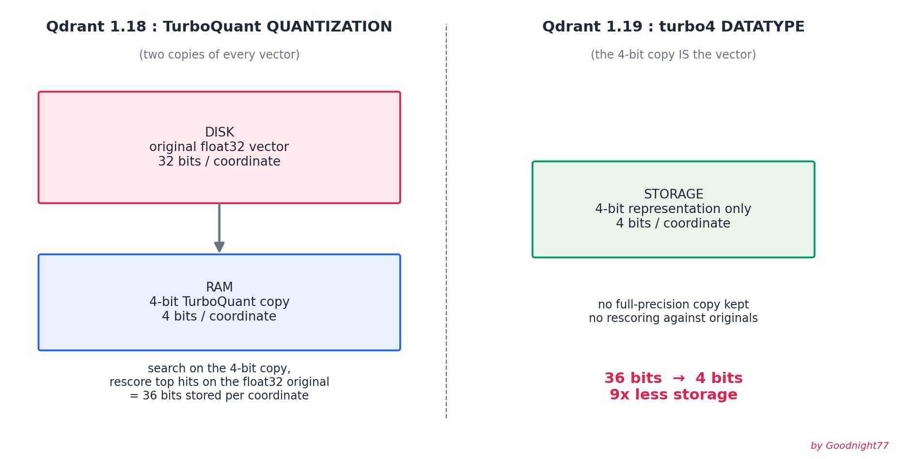
Two-copy quantization in 1.18 vs the turbo4 datatype in 1.19

In 1.19, turbo4 is a datatype, like float32 or float16. When you pick it, Qdrant applies the TurboQuant compression at write time and keeps ONLY the 4-bit result. No full-precision original. 36 bits become 4 bits, that’s the 9x storage reduction the release notes talk about.

think of it like this: in 1.18 you kept the RAW photo and a compressed JPEG next to it “just in case”. in 1.19 you decide the JPEG is good enough and delete the RAW. you save a ton of space, but you can never go back to the original pixels.

and that “never go back” part is exactly the trade-off. Without the full-precision copy, Qdrant cannot rescore top candidates against the originals. You lose the correction step. So:

if disk cost is your problem (huge collections, ColBERT-style multivectors where every document stores many vectors) → turbo4 datatype
if maximum recall is your priority → keep float32 (or float16) storage and put TurboQuant quantization on top, exactly like in 1.18

Here’s what it looks like in code, two collections, one line of difference:

from qdrant_client import QdrantClient, models

client = QdrantClient(url="http://localhost:6333")

# baseline: classic full-precision storage
client.create_collection(
    collection_name="demo_float32",
    vectors_config=models.VectorParams(
        size=1024,
        distance=models.Distance.COSINE,
    ),
)

# 1.19: 4-bit storage, no full-precision copy
client.create_collection(
    collection_name="demo_turbo4",
    vectors_config=models.VectorParams(
        size=1024,
        distance=models.Distance.COSINE,
        datatype=models.Datatype.TURBO4,   # <-- the whole feature
    ),
)

I ran both collections against the same 5,000 synthetic vectors (1024 dims) and measured recall@10 against an exact numpy brute-force search. The chart below shows the results:

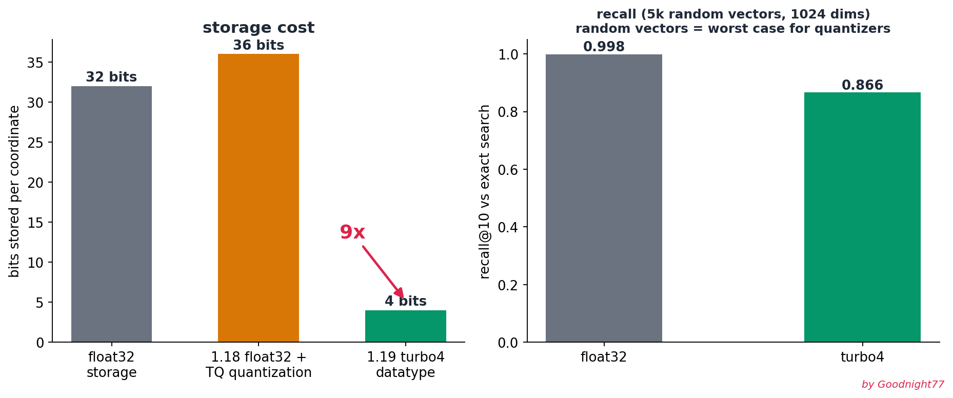
Measured storage and recall comparison between float32 and turbo4

on the left: bits stored per coordinate, 32 for plain float32, 36 for the 1.18 two-copy setup, 4 for turbo4. on the right: recall@10 measured on my run, 0.998 for float32 vs 0.866 for turbo4, a 13-point gap. one important caveat about that gap: random gaussian vectors are the worst possible case for any quantizer. real embedding models produce structured, correlated vectors, and TurboQuant is much closer to full precision on them. always benchmark on YOUR embeddings before deciding (the script to do exactly that is in the repo).

one more nice option the docs mention: you can stack 1-bit TurboQuant quantization ON TOP of turbo4 storage. the search runs on the tiny 1-bit index, and rescoring happens against the 4-bit vectors instead of float32 originals. much cheaper than 1-bit + float32, with rescoring precision somewhere in between. The decision guide below summarizes the three setups:

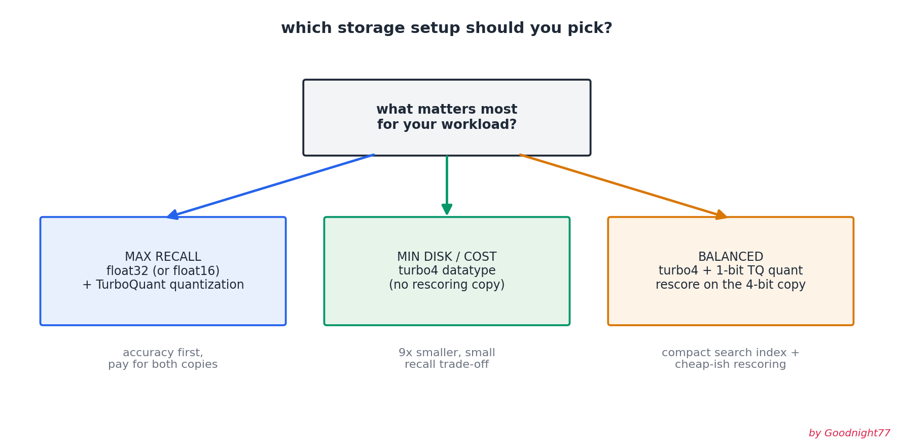
Decision guide: float32 + quantization vs turbo4 vs turbo4 + 1-bit

note: turbo4 works for dense vectors and multivectors only, sparse vectors can’t use it.

2. Memory Tiers: one knob instead of three

If you’ve configured Qdrant for production before, you’ve met the trio: on_disk for vectors, always_ram for quantized vectors, on_disk_payload for payloads. three different names, three slightly different behaviors, for what is really ONE question: where does this data live, RAM or disk?

1.19 replaces all of them with a single memory parameter that works identically on every component of a collection: vectors, the HNSW index, quantized vectors, the sparse index, payloads, and payload indexes.

There are exactly three tiers:

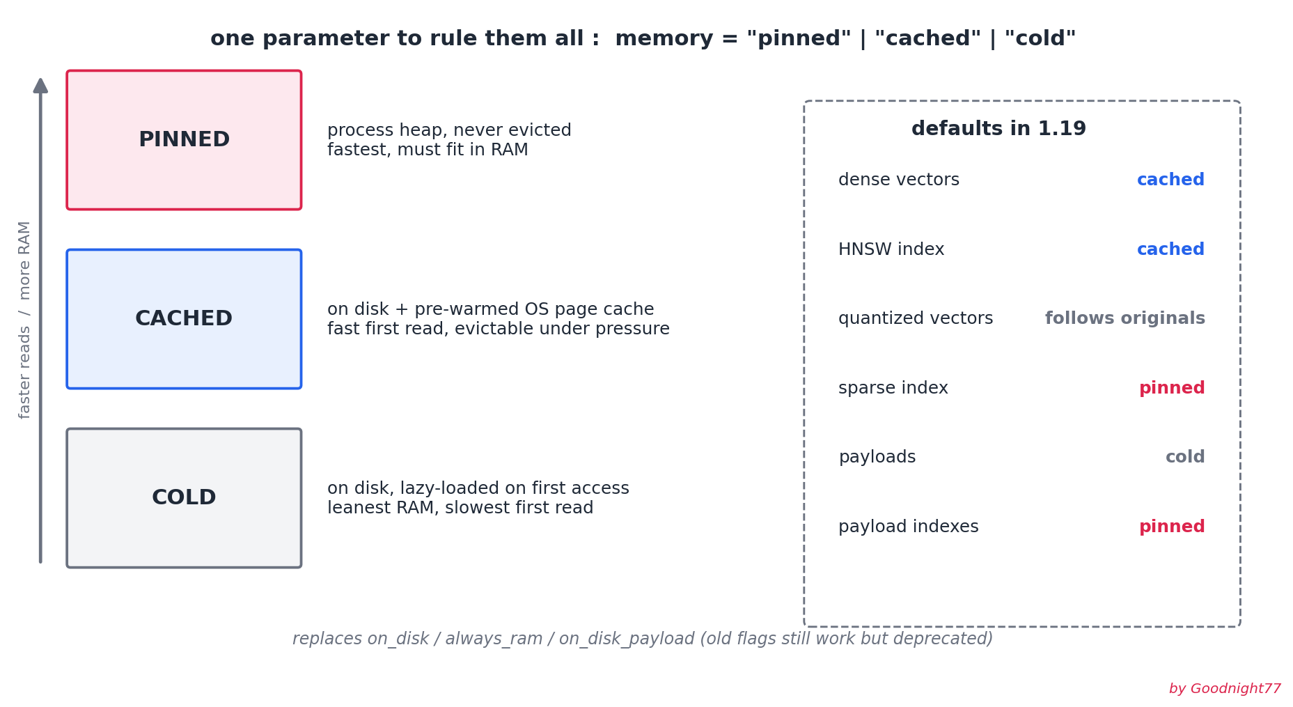
The three memory tiers: pinned, cached, cold

pinned: loaded onto the heap, never evicted. fastest, but the structure must fit in RAM at all times
cached: lives on disk, but Qdrant pre-warms the OS page cache at startup, so the first read is already fast. under memory pressure the OS can evict it
cold: lives on disk, loaded lazily on first access. cheapest RAM, slowest first query

cached and cold are actually the same memory-mapped file underneath, the only difference is whether Qdrant warms the page cache proactively at startup. and the OS treats both the same under pressure, cached gets no eviction priority.

Here’s a disk-first configuration where every component gets an explicit tier:

client.create_collection(
    collection_name="demo_memory_tiers",
    vectors_config=models.VectorParams(
        size=1024,
        distance=models.Distance.COSINE,
        memory=models.Memory.CACHED,       # originals: warm disk cache
    ),
    hnsw_config=models.HnswConfigDiff(
        memory=models.Memory.COLD,         # graph links: lazy-load
    ),
    quantization_config=models.ScalarQuantization(
        scalar=models.ScalarQuantizationConfig(
            type=models.ScalarType.INT8,
            memory=models.Memory.PINNED,   # compressed copy: locked in RAM
        ),
    ),
    payload=models.PayloadStorageParams(
        memory=models.Memory.CACHED,       # payload JSON: warm disk cache
    ),
)

The logic behind this combo: the quantized copy is tiny, so pinning it is cheap, and it’s the thing every single search touches, keep it on the heap. The float32 originals are only read to rescore the top candidates, cached keeps those reads warm without locking gigabytes. The HNSW graph on cold gives you a leaner startup, switch it to cached if cold-start p99 matters to you.

two gotchas worth knowing: pinned is rejected for dense vectors and payloads (they only support memory-mapped representations, so cached is their fastest tier), and the old flags still work but are deprecated, so migrate when you can. 1.19 also unlocked combos that didn’t exist before: HNSW links can now be pinned, sparse indexes gained a cached tier, and quantized vectors can be placed independently of the originals.

This one is for everyone running multi-tenant BM25 / sparse search (if multitenancy in Qdrant is new to you, I covered the whole topic, payload partitioning, tiered multitenancy, tenant promotion, in this article).

BM25 scoring relies on IDF (inverse document frequency): rare terms get more weight than common ones. To compute it you need two numbers, the total document count and how many documents contain each term. Until now, Qdrant computed those statistics over the WHOLE dataset in each shard.

Why is that a problem? Look at the diagram:

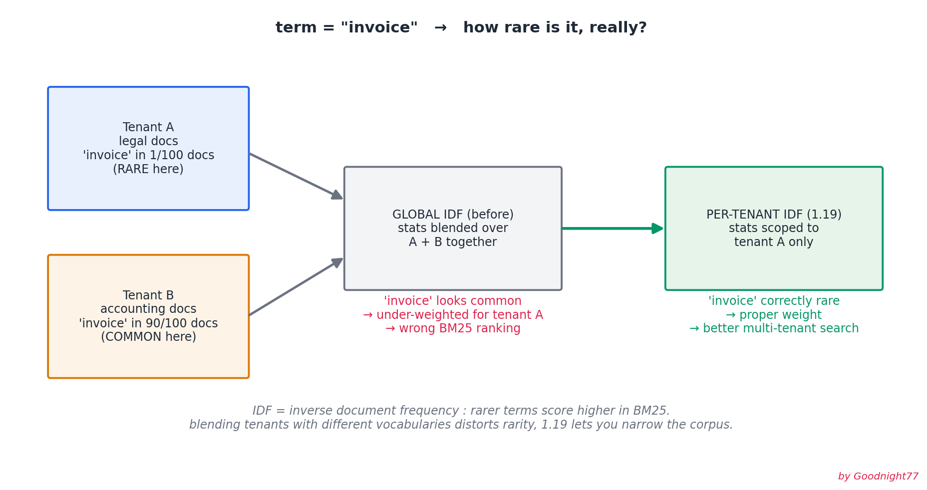
Global IDF blends tenant vocabularies and distorts term rarity

Tenant A stores legal documents where the word “invoice” is rare and highly meaningful. Tenant B stores accounting documents where “invoice” appears in basically every file. Blend both populations into one statistic and “invoice” looks common, so when tenant A searches, the term gets under-weighted and their ranking suffers, even though inside THEIR data it’s a strong signal.

1.19 lets you narrow the corpus the IDF statistics are computed over, down to a single tenant, so term rarity reflects that tenant’s actual vocabulary. If you filter by group_id anyway (which you should in a multi-tenant setup), scoping the IDF to the same tenant is the natural next step. Check the multitenancy docs for the exact query syntax for your client.

4. Filtering: prefix matching and slicing

two new filtering tools, both small on the surface, both solving real operational pain.

Prefix matching on keyword fields

Keyword indexes store values verbatim for exact matching, which is exactly right for identifiers: URLs, file paths, SKUs. But “give me every point whose URL starts with https://qdrant.” was impossible without either a full payload scan or switching to a text index, which tokenizes the value and destroys exact matching.

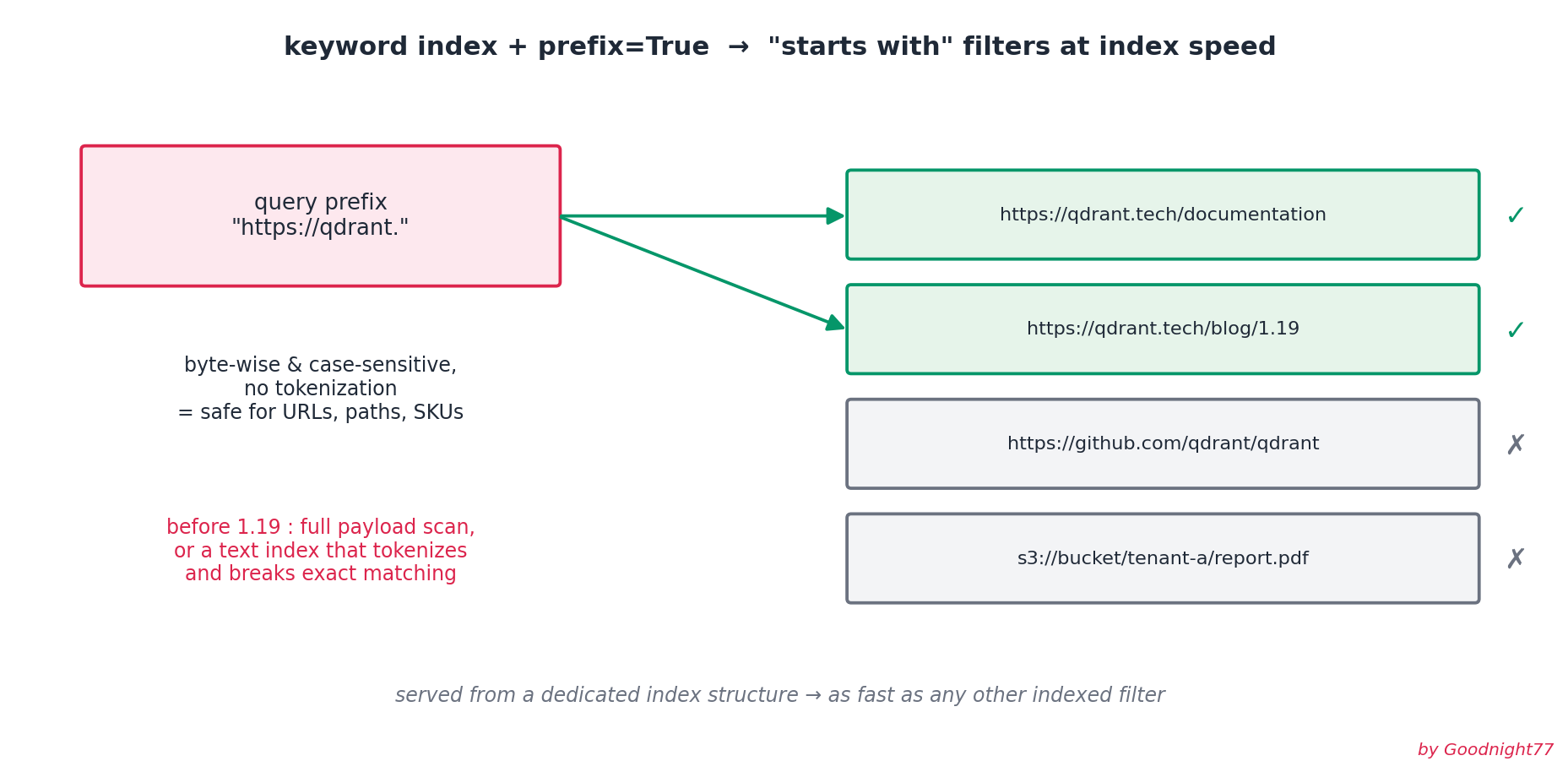
Prefix matching on keyword indexes

1.19 adds a prefix option to the keyword index and a matching prefix condition in filters. The queries are served from a dedicated index structure, so they run at the same speed as any other indexed filter:

# build the index with prefix support
client.create_payload_index(
    collection_name="demo_prefix",
    field_name="url",
    field_schema=models.KeywordIndexParams(
        type=models.KeywordIndexType.KEYWORD,
        prefix=True,   # <-- one flag
    ),
)

# then filter with the new condition
client.scroll(
    collection_name="demo_prefix",
    scroll_filter=models.Filter(
        must=[
            models.FieldCondition(
                key="url",
                match=models.MatchPrefix(prefix="https://qdrant."),
            )
        ]
    ),
)

matching is byte-wise and case-sensitive, same rules as exact keyword matching, no tokenization surprises.

The slice condition

my personal favorite of the release. The slice condition splits a collection into deterministic, disjoint subsets using a stable hash of the point ID:

a point belongs to slice index of total if hash(id) % total == index

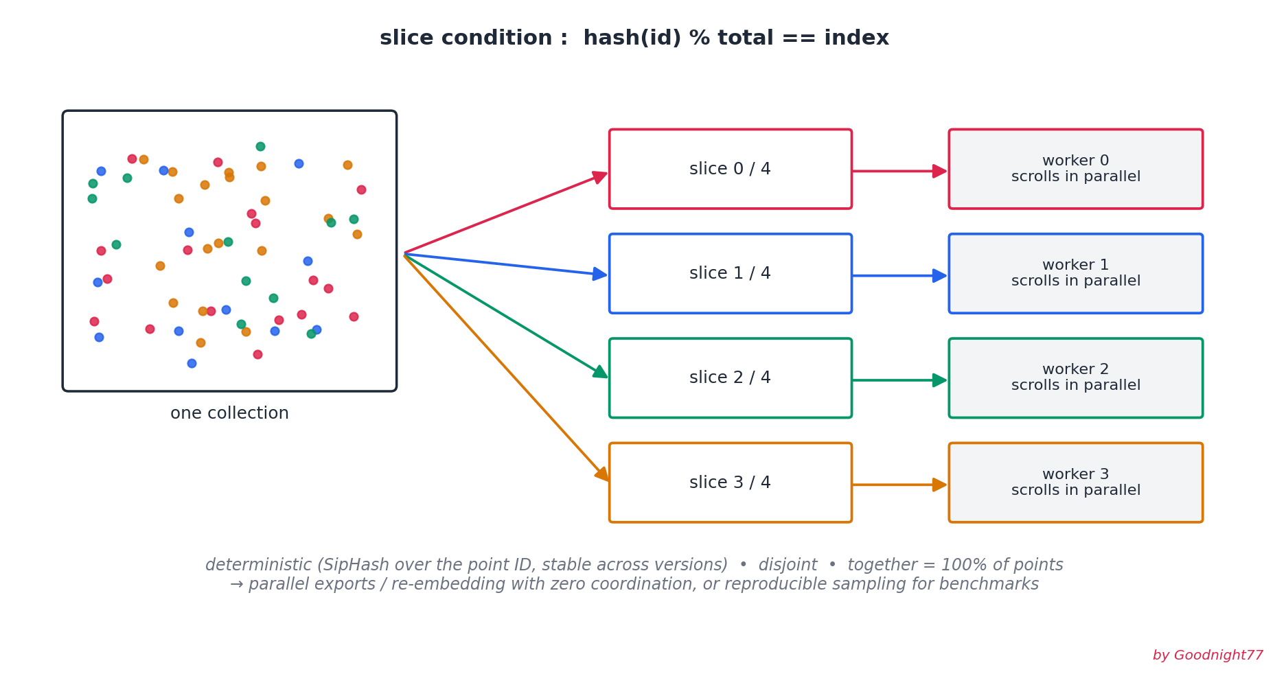
The slice condition partitions a collection into disjoint subsets for parallel workers

why is this cool? two patterns that used to be painful become trivial:

parallel processing. you want to export, migrate, or re-embed an entire collection. before, workers had to coordinate offsets or split ID ranges manually. now: worker 0 scrolls slice 0/4, worker 1 scrolls slice 1/4, and so on. zero coordination, no overlap, full coverage guaranteed.

# each worker runs this with its own slice_index, nothing else to coordinate
points, offset = client.scroll(
    collection_name="demo_slices",
    scroll_filter=models.Filter(
        must=[
            models.SliceCondition(
                slice=models.Slice(index=worker_id, total=4)
            )
        ]
    ),
    limit=500,
    offset=offset,
)

reproducible sampling. unlike random sampling, the same slice ALWAYS returns the same points. the hash is SipHash-2-4 with a zero key over the ID bytes and Qdrant guarantees it won’t change across versions. that makes slices perfect for recall benchmarks, train/test splits, and canary rollouts. bonus detail from the docs: slices with different totals are correlated, slice 0 of total=4 is always a subset of slice 0 of total=2, so you can grow or shrink your sample without reshuffling.

I verified all three properties (disjoint, complete, deterministic) with a script in the repo, 4 threads scanning 2,000 points in parallel: 0 overlap, 100% coverage, identical re-reads.

Also in this release

quick hits worth knowing:

Resource quotas: cap how much memory and disk a node can use, so it degrades instead of dying
Replica read affinity: pin a user’s reads to the same replica with an X-Qdrant-Route-Affinity header, killing the “I just wrote it, why can’t I read it” inconsistency between replicas
Language-neutral BM25: turn off English stemming and stopwords, better for code, product IDs, and multilingual text
Faster faceting on high-cardinality fields
breaking: the legacy /search, /recommend, and /discover endpoints are REMOVED. if you still use them, migrate to the unified /query API before upgrading
the Web UI got live resharding progress, a Collection Visualizer that now handles tens of thousands of points, and payload index management from the interface

Upgrading: go one minor version at a time (1.17.x → 1.18.x → 1.19.0). Qdrant Cloud does this automatically when you pick the target version.

Try it yourself

everything in this post is reproducible. the companion project contains:

01_turbo4_vs_float32.py: builds both collections, measures recall@10 vs exact search
02_memory_tiers.py: a fully-tiered collection with the config verified back from the server
03_prefix_matching.py: prefix index + filters on URLs and S3 paths
04_slice_parallel_scroll.py: 4 parallel workers proving disjointness, coverage, and determinism

spin up Qdrant with docker compose up -d, then python scripts/01_turbo4_vs_float32.py. no API keys, no embedding model downloads, the whole thing runs in under a minute.

definitions

datatype vs quantization: a datatype defines how the ORIGINAL vectors themselves are stored (float32, float16, uint8, turbo4). quantization creates a SEPARATE compressed representation alongside the originals. turbo4 blurs the line: it applies quantization math at the datatype level
rescoring: after searching on a compressed representation, re-ranking the top candidates using the original full-precision vectors to correct small errors. impossible with turbo4 because the originals no longer exist
memory-mapped file (mmap): a file on disk that the OS presents as if it were memory. reads go through the OS page cache, which is why cached and cold behave the same after warm-up
IDF (inverse document frequency): the part of BM25 that boosts rare terms. computed from document counts, which is why the corpus you compute it over matters
SipHash-2-4: a fast, stable hash function. Qdrant uses it (with a zero key) for the slice condition so slice membership never changes between versions

Conclusion

1.19 is a “pick your trade-off consciously” release. TurboQuant graduated from a clever cache into a first-class storage format, and the question it forces is honest: do you actually need those float32 originals, or are you paying 9x storage for a rescoring step your recall budget doesn’t require? Memory tiers turn a scattered set of flags into one vocabulary you can reason about, and slice + prefix quietly fix two operational headaches (parallel exports and identifier filtering) that everyone has hacked around at some point. My advice: run the turbo4 recall benchmark on YOUR embeddings first, it’s a one-line config change to test and the script is right there. If the recall holds, that’s the cheapest 9x you’ll get this year.

References :

Share this article:

(END)