Vector search systems like Qdrant are designed to handle a very specific problem: searching through millions of high-dimensional embeddings with low latency. To understand how Qdrant achieves this, you need to look beyond the API and examine how data is stored, distributed, and queried internally.
Interactive Qdrant Anatomy Viewer
When I first worked with Qdrant, what stood out was how much complexity sits behind a simple API, this article is my attempt to break a bit that complexity down into clear building blocks so that it would help others understand the inner workings of qdrant, especially those who are new to vector databases
Components
Collections
a collection is the top level container in Qdrant
it’s similar to a table in a relational database, except each row is a high-dimensional vector instead of a tuple of scalar values.
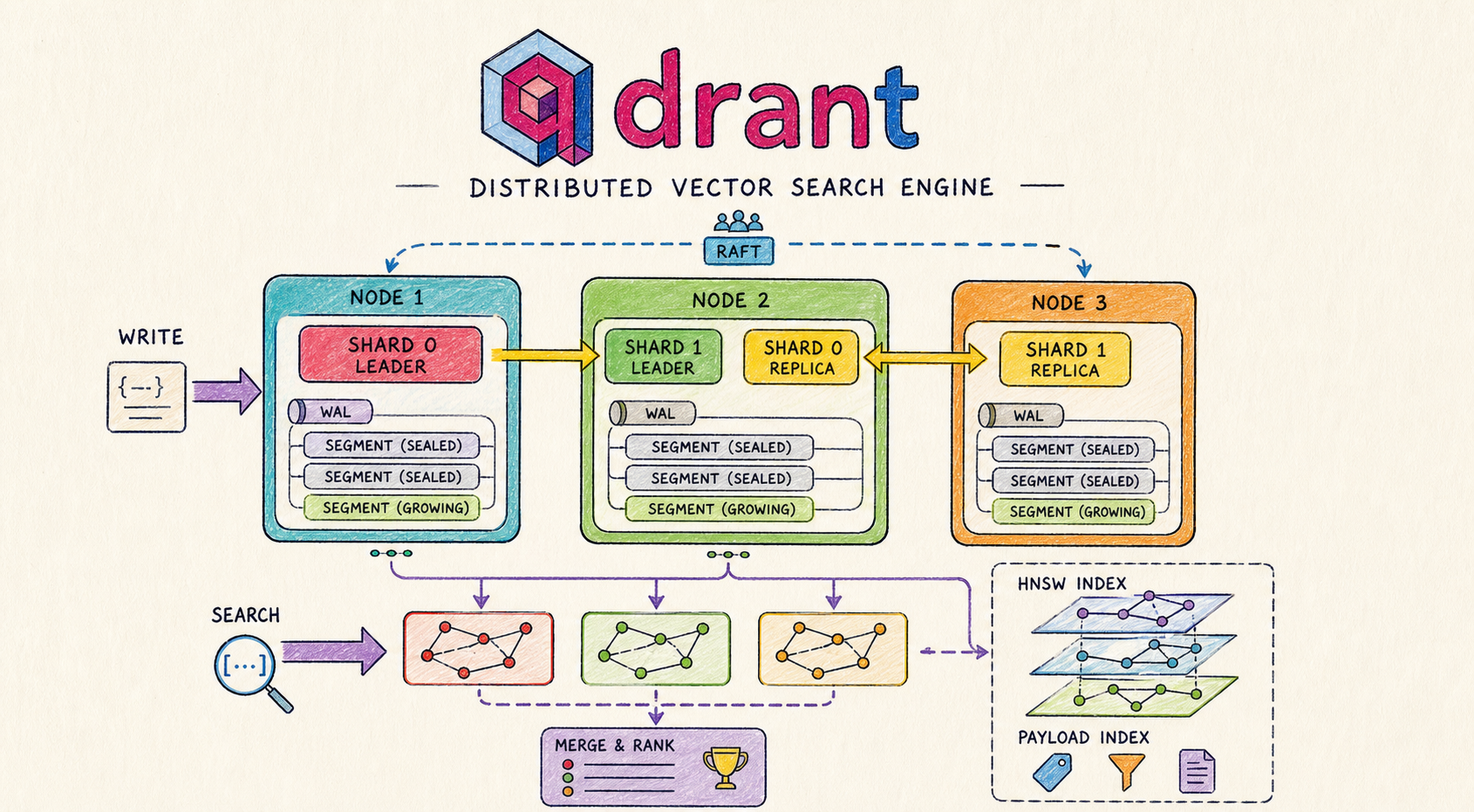
in diagram the red boxes appear inside every node
a single collection is a logical namespace that spans entire cluster even though its data is physically scattered across machines
when create one you fix three things up front;
- vector dimensionality of the vectors it will hold (384, 768, 1536)
- the distance metrics used to compare them (cosine , dot product)
- the indexing parameters that govern search behavior every vector inserted afterward must follow this schema once dim is fixed, memory layout, SIMD vectorization and graph construction call all be specialized
Point
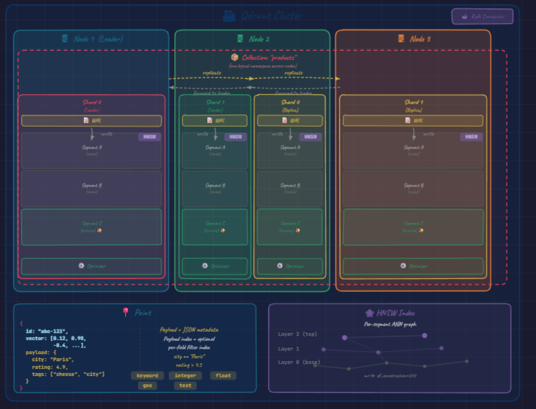
this is the atomic unit stored inside a collection, a point is a small struct an id , a vector (embedding ) and payload which you can call it metadata : a JSON metadata like
{ "city": "Paris", "rating": 4.7, "tags": ["visites","cheese", "parfum"] }this payload is what turns our vector db from pure similarity engine into something usable for production retrieval, because it lets you constrain to subsets of data (“nearest neighbors among 4 star paris restaurants”) rather than running unfiltered nearst neighbor over millions of vectors and post filtering the finding results
Shards
a collection is a logical concept ; but on the other hand shard is a physical manifestation. each shard is a horizontal partition holding a disjoint subset of the collection’s points in the diagram, our collection is divided into 2 shards
- shard 0 (red)
- shard 1 (green)
by default (Auto sharding) qdrant hashes the point’s id to pick a shard, plain hash-based partitioning (modulo over shard count), not consistent hashing in the Dynamo/Cassandra sense. qdrant also supports Custom sharding, where you define shard keys explicitly (commonly used for tenant isolation in multitenant setups). this is the mechanism by which qdrant scales horizontally, doubling the number of shards allows the system to scale horizontally by distributing data and write load, in ideal conditions, this improves throughput but actual gains depend on network and query patterns.
Segments
inside each shard you will find a stack of segments; the actual storage units where vectors live on disk, diagram shows 3 per shard
and labels matters Segment A (sealed), Segment B (sealed), and Segment C (growing) ✨
segments follows LSM-tree-like discipline:
- if you inserted new points they will always goes into growing (mutable) segment
- once it reaches a size threshold, it is sealed (frozen as immutable)
- a new growing segments takes its place sealed segments are what get heavily indexed, mutable ones use simples structures because they are constantly chnaging
WAL (write ahead log)
the durability guarantee: every write is appended to the log before it touches a segment, so a crash mid-write doesn’t lose data. note that the WAL is per-shard, not per-node, each shard owns its own WAL (the diagram simplifies this by drawing one WAL at the top of each node).
Optimizer
Optimizer (on the right down of the diagram), is the background process that stops the segment stack from growing too much:
it merges small segments into larger ones, builds the HNSW graph on newly sealed segments, and
garbage-collects vectors that have been logically deleted. Without the optimizer, search would slow linearly with insert volume.
Nodes
a node is a single Qdrant instance (usually a machine or container), it hosts shards and handles storage, indexing and query execution. the diagram shows three of them:
- Node 1 (teal, marked Leader)
- Node 2 (green)
- Node 3 (orange)
Nodes are the unit of physical infrastructure; everything above them (collections, shards, replicas) is logical and gets mapped onto nodes
by the cluster orchestration layer.
Each node runs its own
WAL, its ownsegmentstore, and its own copy of the cluster’s metadata. What turns three independent processes into one coherent cluster is theRaft Consensusmodule shown at the top right of the diagram.
Raft
Raft is used to maintain cluster metadata not the actual vector data, it ensures all nodes agree on
- which collections exist
- which nodes are alive
- where each shard and replica are placed, and which replica is currently the leader for each shard.
one node is elected the Raft leader (Node 1 in the diagram), and all metadata changes flow through it. If that leader dies, the remaining nodes hold an election and a new
leader takes over, typically within a few seconds.
a critical distinction: Raft governs metadata consensus, not data replication. The actual vectors don’t go through Raft, that would be far
too slow for a database designed around bulk vector ingestion.
Data replication uses a separate, lighter mechanism described in the next section.
that mechanism isn’t always fire-and-forget: qdrant exposes per-request write consistency modes. The default forwards writes
to replicas asynchronously, but you can require the leader to wait for replica acknowledgement (majority / all) when you need stricter guarantees, trading latency for durability.
Qdrant scales using two mechanisms:
Replication and distribution
this is where the diagram’s layout becomes most informative. the four shard-blocks are placed across the three nodes like this:
- Node 1 → Shard 0 (Leader), red block
- Node 2 → Shard 1 (Leader) (green) + Shard 0 (Replica) (yellow)
- Node 3 → Shard 1 (Replica) (yellow)
this arrangement encodes Qdrant’s two orthogonal scaling axes simultaneously:
- Sharding (Shard 0 vs Shard 1) splits the data so no single node stores or searches the full collection.
- Replication (Leader vs Replica) duplicates each shard onto a second node, so any single node failure still leaves every shard reachable.
The yellow replicate arrows in the diagram represent the asynchronous replication stream that keeps replicas in sync with their leaders.
How writes flow
- Exactly one replica per shard is the leader at any given time.
- Writes hit the leader → appended to its WAL → applied to the growing segment → forwarded to follower replicas.
- Reads can be served by any replica (leader or follower), so read throughput scales with the replication factor.
- If the leader node dies, the cluster (via Raft) promotes a surviving replica to leader and writes resume.
Replication factor trade-off
The replication factor is configurable per collection:
| Factor | Failure tolerance | Cost |
|---|---|---|
| 2 (shown in diagram) | 1 node failure | base |
| 3 | 2 node failures | more storage, more write traffic |
Higher factor → stronger fault tolerance, at the cost of more storage and more network traffic on writes.
Indexing and retrieval
all the structure described so far exists to make one operation fast:
given a query vector, find the K most similar vectors in the collection. The piece that delivers that speed is the HNSW Index, shown in the bottom-right panel of the diagram with its characteristic three-layer graph illustration.
HNSW (Hierarchical Navigable Small World)
HNSW is the algorithm Qdrant uses for approximate nearest-neighbor search.
Layered graph structure:
- Layer 2 (top) → handful of “highway” nodes
- Layer 1 (middle) → more nodes, denser connectivity
- Layer 0 (base) → every point in the segment
This layering reduces search complexity from linear to roughly logarithmic.
How a search runs:
- Start at a random entry point in the top layer.
- Greedily walk toward the query vector.
- Drop down a layer, walk again.
- Repeat until you finish on the base layer with a fine-grained search.
Result: O(log N) expected complexity (per the HNSW paper) instead of the linear cost of brute-force comparison.
Tuning parameters (visible at the bottom of the diagram panel):
m = 16→ graph connectivity (higher = better recall, more memory)ef_construction = 200→ build thoroughness (higher = better recall, slower index build)
Easy-to-miss but important details:
- HNSW is built per segment, not per shard. Each sealed segment has its own independent graph.
- A shard search fans out across all its segments in parallel and merges results.
- This is why the optimizer’s segment-merging matters: fewer, larger segments → fewer parallel sub-searches → better cache behavior.
Payload Index
The Payload Index (yellow in the bottom panel) is a separate structure that supports filtered search. For a query like city == "Paris" AND rating > 4.5, Qdrant does not blindly run nearest-neighbor and filter after. A query planner picks a strategy based on the filter’s estimated cardinality:
| Strategy | When | What it does |
|---|---|---|
| Pre-filter | Very few matches | Brute-force the filtered subset directly |
| Filterable HNSW | Medium cardinality | Push the filter into the graph traversal — walk only considers points satisfying the predicate |
| Post-filter | Very loose filters | Run normal HNSW, drop non-matching points after |
Supported field types: keyword, integer, float, geo, full-text — each with its own internal structure. The payload index also feeds the cardinality estimates the planner uses.
Putting it all together
A single search request follows this path:
- Request hits any node.
- Node consults cluster metadata → figures out which shards hold candidate data.
- Sub-queries dispatched in parallel to one replica per relevant shard (local replicas preferred).
- Each replica runs
HNSW + payload-filteracross its segments. - Partial results stream back → coordinator merges into the final top-K.
With well-tuned shard and segment counts, the full round trip lands in the single-digit millisecond range — even on collections of hundreds of millions of vectors. That’s the engineering payoff all the architectural complexity above exists to deliver.
System view
A full request follows this path:
- write → WAL → segment (growing → sealed)
- data is distributed across shards
- shards are replicated across nodes
- search query is sent to all relevant shards
- each shard runs HNSW + filtering
- results are merged into final top-K
This combination is what enables low-latency search at scale.
Final thoughts
Qdrant’s performance doesn’t come from a single trick, but from how multiple components work together: segmentation, sharding, replication, and graph-based indexing.
each piece solves a specific problem, but the real strength is in how they combine into a system that scales while keeping latency low
understanding this architecture makes it easier to:
- tune performance
- debug behavior
- design similar systems
References
- Qdrant internals
- Qdrant distributed deployment
- Qdrant Documentation
- Qdrant Cloud Sign Up
- Subscribe to the Qdrant Newsletter

(END)